Plotting

A-scans

plot_Ascan.py

This module uses matplotlib to plot the time history for the electric and magnetic field components, and currents for all receivers in a model (each receiver gets a separate figure window). Usage (from the top-level gprMax directory) is:

python -m tools.plot_Ascan outputfile

where outputfile is the name of output file including the path.

There are optional command line arguments:

• --outputs to specify a subset of the default output components (Ex, Ey, Ez, Hx, Hy, Hz, Ix, Iy or Iz) to plot. By default all electric and magnetic field components are plotted.

• -fft to plot the Fast Fourier Transform (FFT) of a single output component

For example to plot the Ez output component with it’s FFT:

python -m tools.plot_Ascan my_outputfile.out --outputs Ez -fft

B-scans

plot_Bscan.py

gprMax produces a separate output file for each trace (A-scan) in the B-scan. These must be combined into a single file using the outputfiles_merge.py module (described in the other utilities section). This module uses matplotlib to plot an image of the B-scan. Usage (from the top-level gprMax directory) is:

python -m tools.plot_Bscan outputfile rx-component

where:

• outputfile is the name of output file including the path

• rx-component is the name of the receiver output component (Ex, Ey, Ez, Hx, Hy, Hz, Ix, Iy or Iz) to plot

Antenna parameters

plot_antenna_params.py

This module uses matplotlib to plot the input impedance (resistance and reactance) and s11 parameter from an antenna model fed using a transmission line. It also plots the time history of the incident and reflected voltages in the transmission line and their frequency spectra. The module can optionally plot the s21 parameter if another transmission line or a receiver output (#rx) is used on the receiver antenna. Usage (from the top-level gprMax directory) is:

python -m tools.plot_antenna_params outputfile

where outputfile is the name of output file including the path.

There are optional command line arguments:

• --tltx-num is the number of the transmission line (default is one) for the transmitter antenna. Transmission lines are numbered (starting at one) in the order they appear in the input file.

• --tlrx-num is the number of the transmission line (default is None) for the receiver antenna (for a s21 parameter). Transmission lines are numbered (starting at one) in the order they appear in the input file.

• --rx-num is the number of the receiver output (default is None) for the receiver antenna (for a s21 parameter). Receivers are numbered (starting at one) in the order they appear in the input file.

• --rx-component is the electric field component (Ex, Ey or Ez) of the receiver output for the receiver antenna (for a s21 parameter).

For example to plot the input impedance, s11 and s21 parameters from a simulation with transmitter and receiver antennas that are attached to transmission lines (the transmission line feeding the transmitter appears first in the input file, and the transmission line attached to the receiver antenna appears after it).

python -m tools.plot_antenna_params outputfile --tltx-num 1 --tlrx-num 2

Built-in waveforms

This section describes the definitions of the functions that are used to create the built-in waveforms, and how to plot them.

plot_source_wave.py

This module uses matplotlib to plot one of the built-in waveforms and it’s FFT. Usage (from the top-level gprMax directory) is:

python -m tools.plot_source_wave type amp freq timewindow dt

where:

• type is the type of waveform, e.g. gaussian, ricker etc…

• amp is the amplitude of the waveform

• freq is the centre frequency of the waveform (Hertz). In the case of the Gaussian waveform it is related to the pulse width.

• timewindow is the time window (seconds) to view the waveform, i.e. the time window of the proposed simulation

• dt is the time step (seconds) to view waveform, i.e. the time step of the proposed simulation

There is an optional command line argument:

• -fft to plot the Fast Fourier Transform (FFT) of the waveform

Definitions

Definitions of the built-in waveforms and example plots are shown using the parameters: amplitude of one, centre frequency of 1GHz, time window of 6ns, and a time step of 1.926ps.

gaussian

A Gaussian waveform.

\[W(t) = e^{-\zeta(t-\chi)^2}\]

where \(\zeta = 2\pi^2f^2\), \(\chi=\frac{1}{f}\) and \(f\) is the frequency.

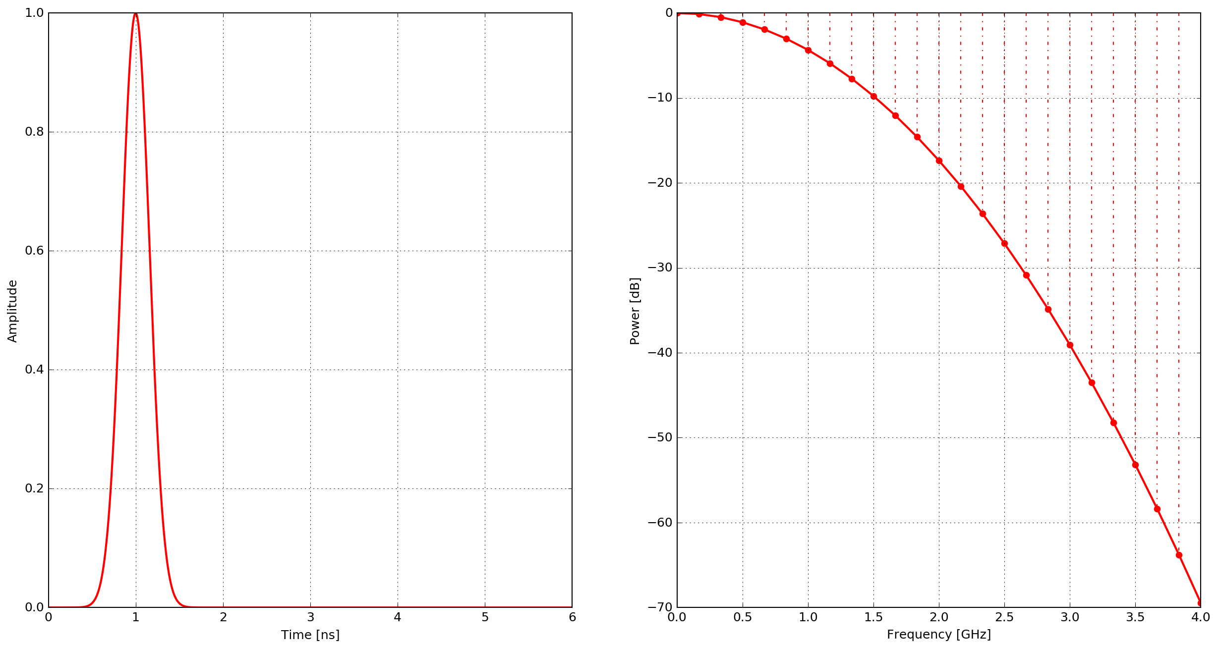
Fig. 7 Example of the gaussian waveform - time domain and power spectrum.

gaussiandot

First derivative of a Gaussian waveform.

\[W(t) = -2 \zeta (t-\chi) e^{-\zeta(t-\chi)^2}\]

where \(\zeta = 2\pi^2f^2\), \(\chi=\frac{1}{f}\) and \(f\) is the frequency.

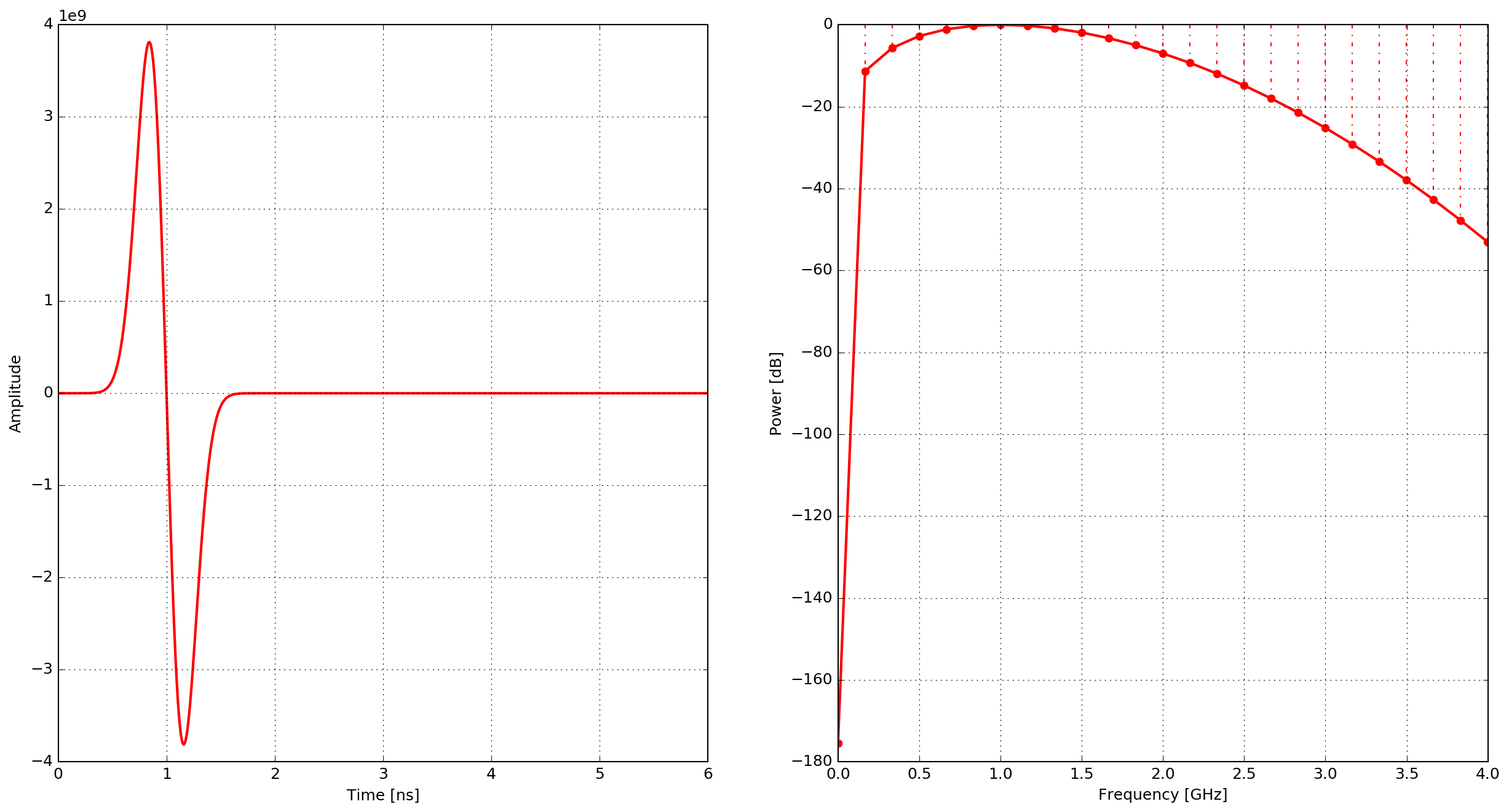
Fig. 8 Example of the gaussiandot waveform - time domain and power spectrum.

gaussiandotnorm

Normalised first derivative of a Gaussian waveform.

\[W(t) = -2 \sqrt{\frac{e}{2\zeta}} \zeta (t-\chi) e^{-\zeta(t-\chi)^2}\]

where \(\zeta = 2\pi^2f^2\), \(\chi=\frac{1}{f}\) and \(f\) is the frequency.

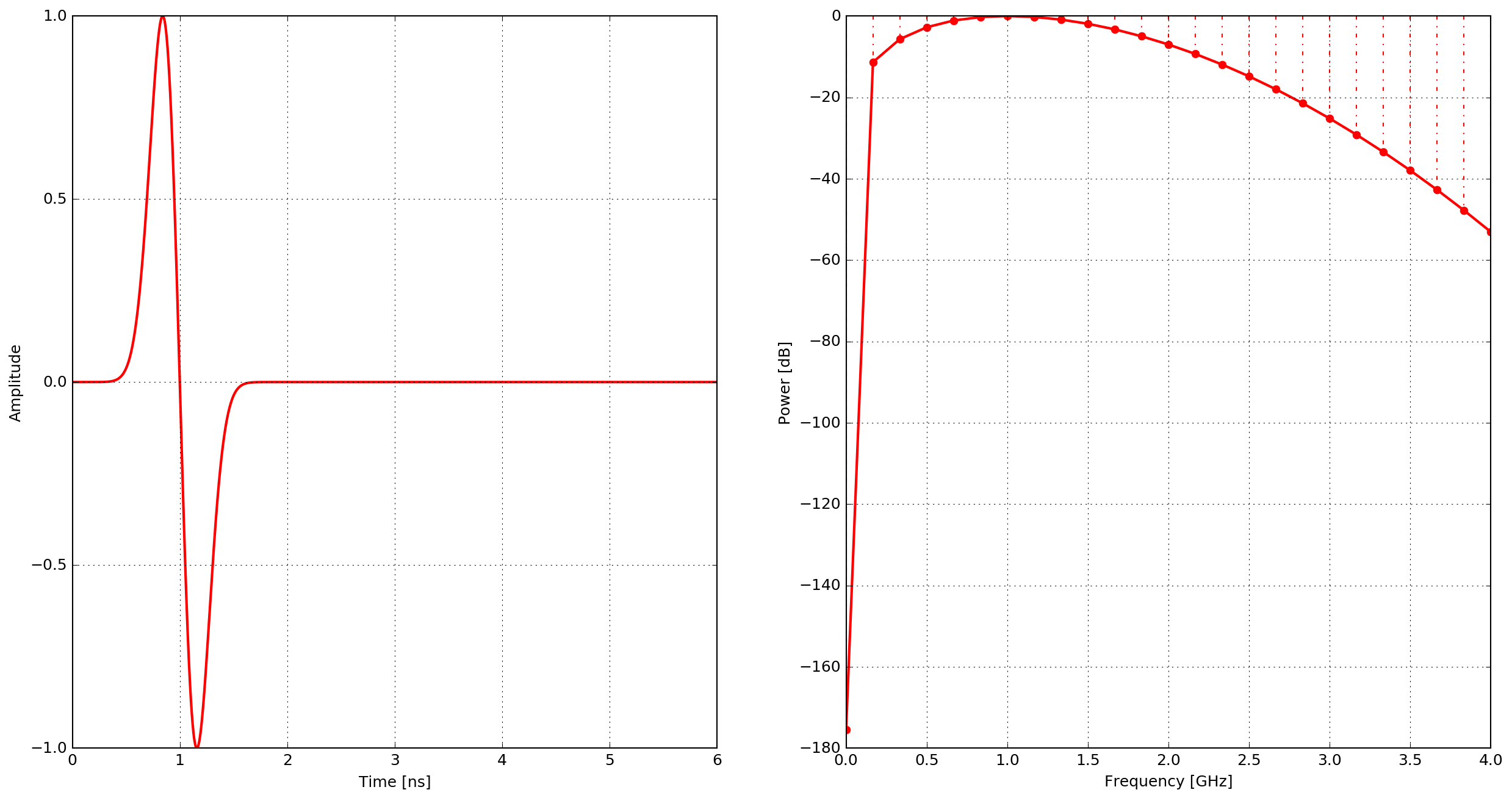
Fig. 9 Example of the gaussiandotnorm waveform - time domain and power spectrum.

gaussiandotdot

Second derivative of a Gaussian waveform.

\[W(t) = 2\zeta \left(2\zeta(t-\chi)^2 - 1 \right) e^{-\zeta(t-\chi)^2}\]

where \(\zeta = \pi^2f^2\), \(\chi=\frac{\sqrt{2}}{f}\) and \(f\) is the frequency.

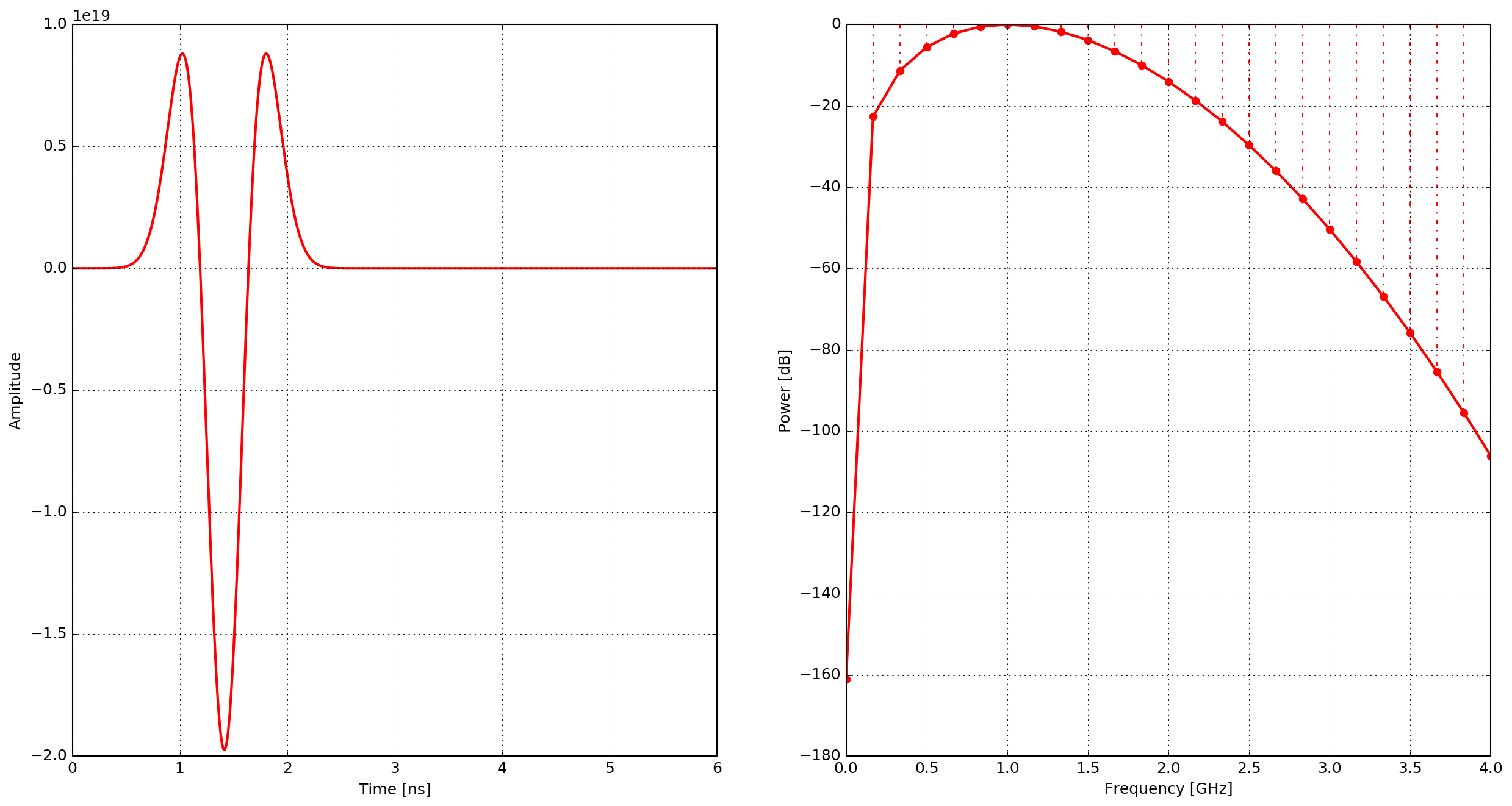
Fig. 10 Example of the gaussiandotdot waveform - time domain and power spectrum.

gaussiandotdotnorm

Normalised second derivative of a Gaussian waveform.

\[W(t) = \left( 2\zeta (t-\chi)^2 - 1 \right) e^{-\zeta(t-\chi)^2}\]

where \(\zeta = \pi^2f^2\), \(\chi=\frac{\sqrt{2}}{f}\) and \(f\) is the frequency.

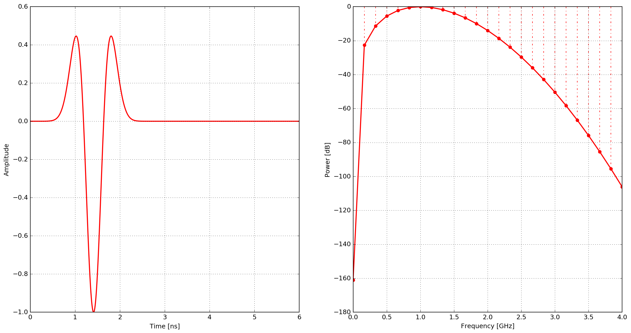
Fig. 11 Example of the gaussiandotdotnorm waveform - time domain and power spectrum.

ricker

A Ricker (or Mexican Hat) waveform which is the negative, normalised second derivative of a Gaussian waveform.

\[W(t) = - \left( 2\zeta (t-\chi)^2 -1 \right) e^{-\zeta(t-\chi)^2}\]

where \(\zeta = \pi^2f^2\), \(\chi=\frac{\sqrt{2}}{f}\) and \(f\) is the frequency.

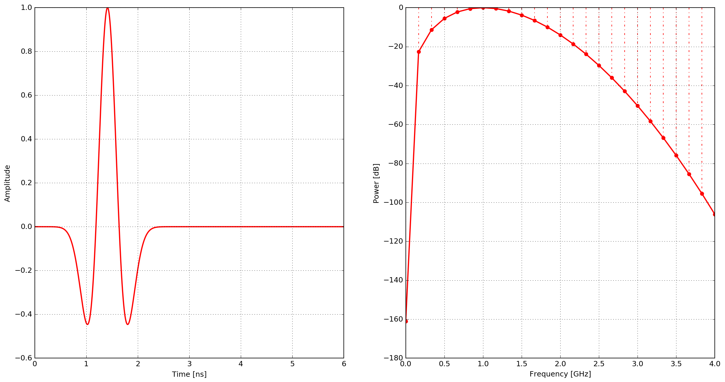
Fig. 12 Example of the ricker waveform - time domain and power spectrum.

sine

A single cycle of a sine waveform.

\[W(t) = R\sin(2\pi ft)\]

and

\[\begin{split}R = \begin{cases} 1 &\text{if $ft\leq1$}, \\ 0 &\text{if $ft>1$}. \end{cases}\end{split}\]

\(f\) is the frequency

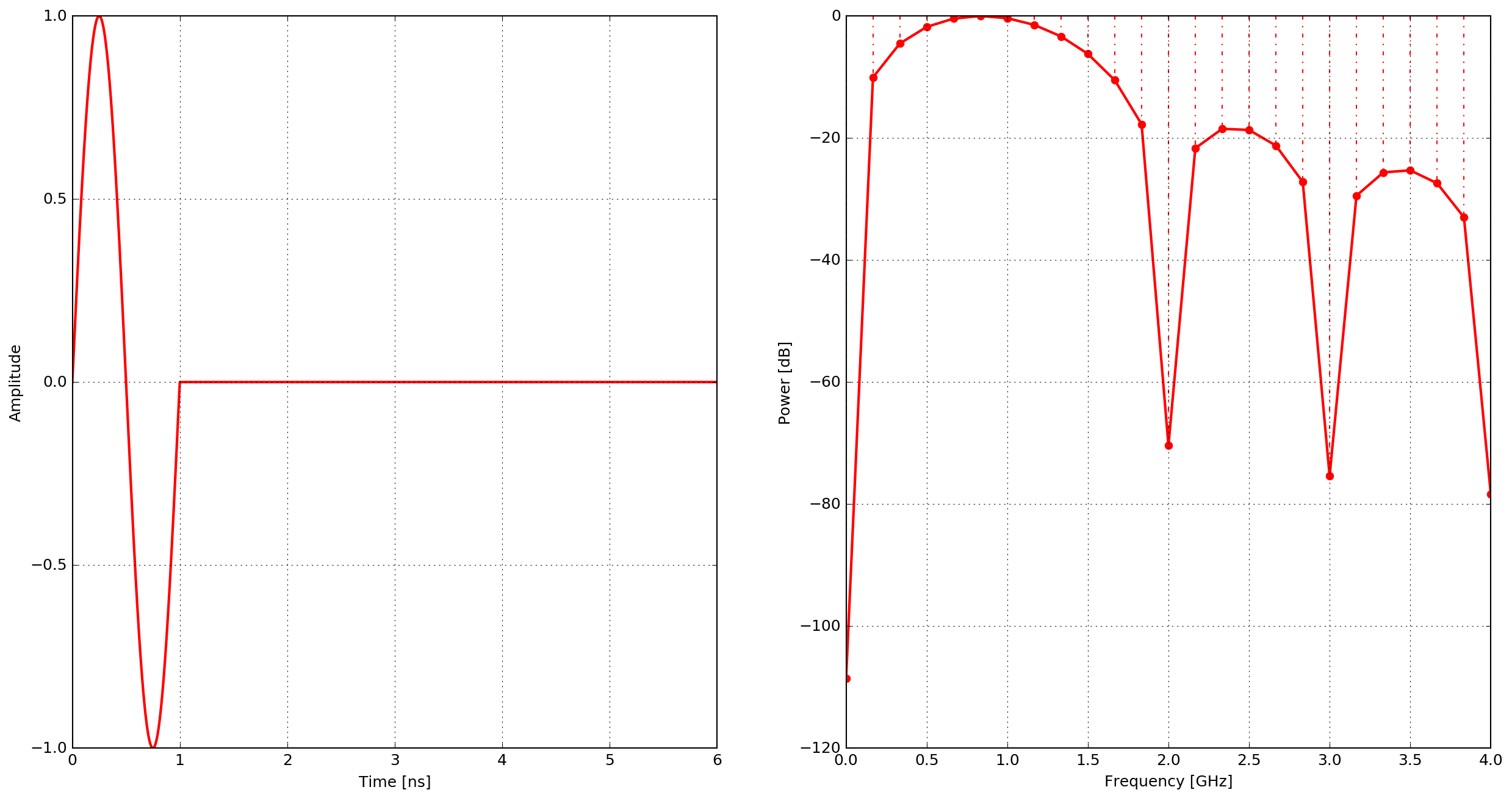
Fig. 13 Example of the sine waveform - time domain and power spectrum.

contsine

A continuous sine waveform. In order to avoid introducing noise into the calculation the amplitude of the waveform is modulated for the first cycle of the sine wave (ramp excitation).

\[W(t) = R\sin(2\pi ft)\]

and

\[\begin{split}R = \begin{cases} R_cft &\text{if $R\leq 1$}, \\ 1 &\text{if $R>1$}. \end{cases}\end{split}\]

where \(R_c\) is set to \(0.25\) and \(f\) is the frequency.

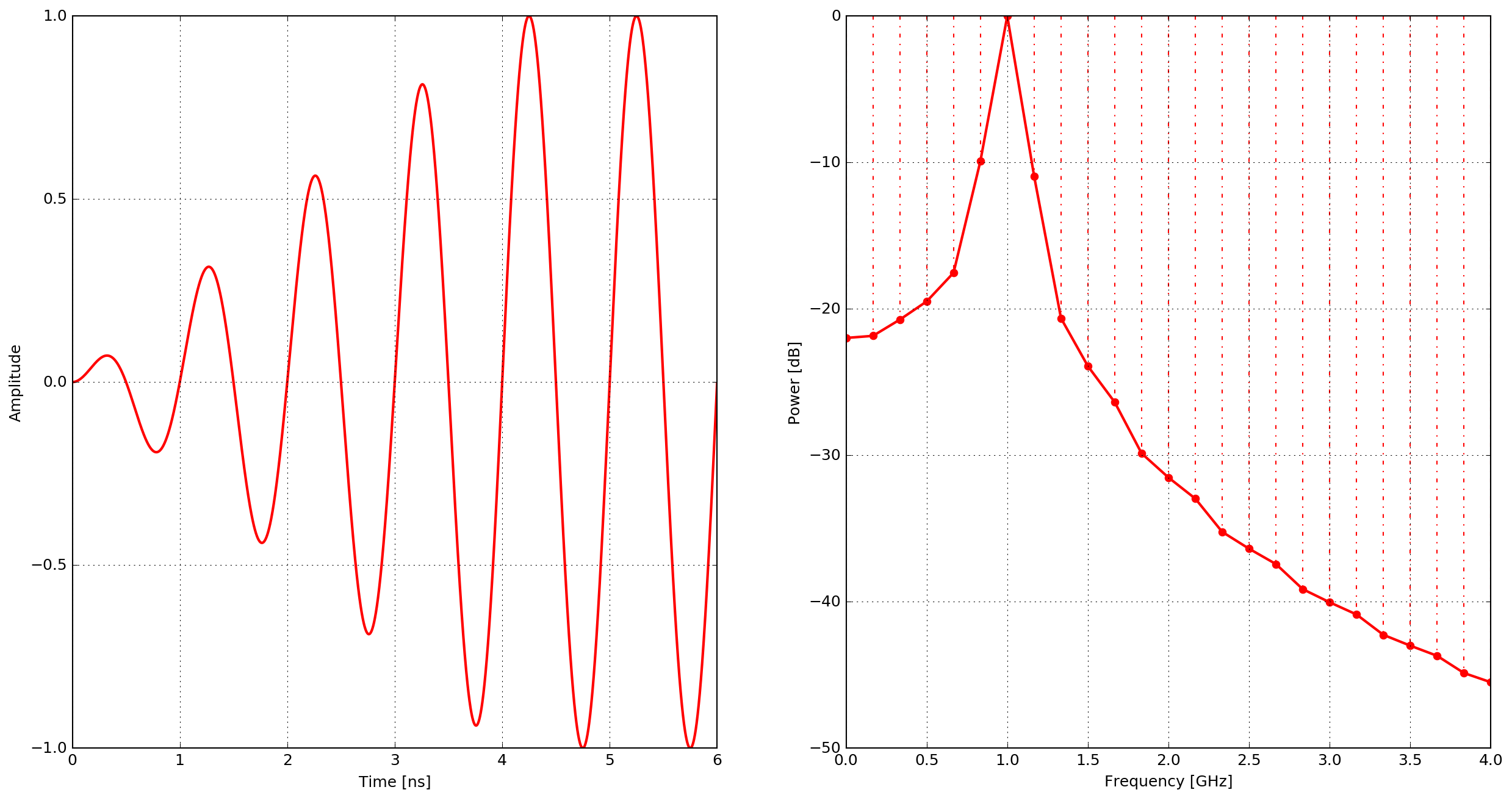
Fig. 14 Example of the contsine waveform - time domain and power spectrum.