Analytical comparisons
This section presents comparisons between analytical solutions and modelled solutions using gprMax.
Hertzian dipole in free space
This example is of a Hertzian dipole, i.e. an additive source (electric current density), in free space.
1#title: Hertzian dipole in free-space
2#domain: 0.100 0.100 0.100
3#dx_dy_dz: 0.001 0.001 0.001
4#time_window: 3e-9
5
6#waveform: gaussiandot 1 1e9 myWave
7#hertzian_dipole: z 0.050 0.050 0.050 myWave
8#rx: 0.070 0.070 0.070
The function hertzian_dipole_fs, which can be found in the analytical_solutions module in the tests sub-package, computes the analytical solution.
Results
Fig. 46 shows the time history of the electric and magnetic field components of the modelled and analytical solutions. The responses completely overlap one another due to their similarity. Therefore, Fig. 47 shows the percentage differences between the modelled and analytical solutions.
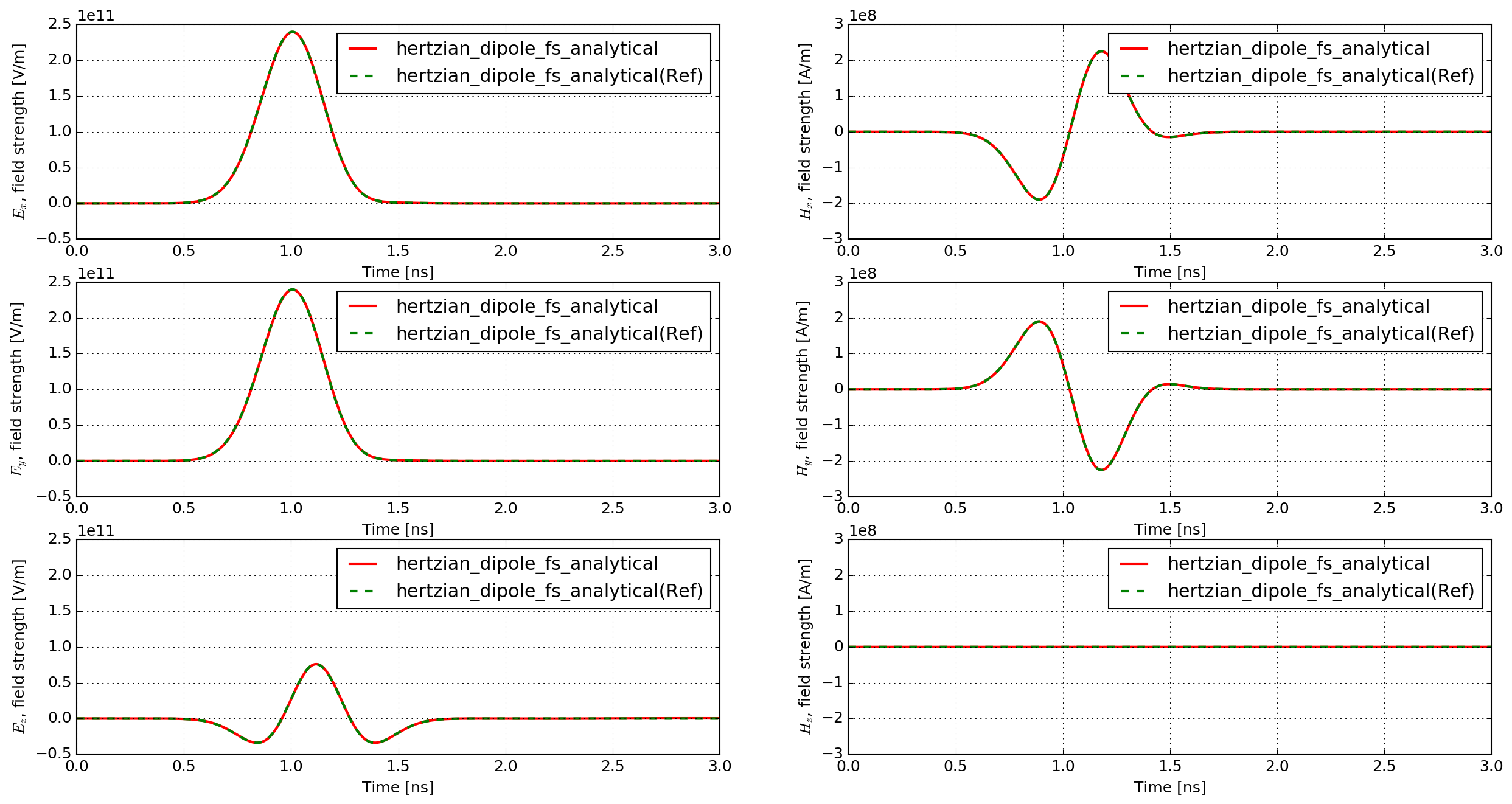
Fig. 46 Time history of the electric and magnetic field components of the modelled and analytical solutions (‘Ref’, in this case, indicates solution calculated from theory).
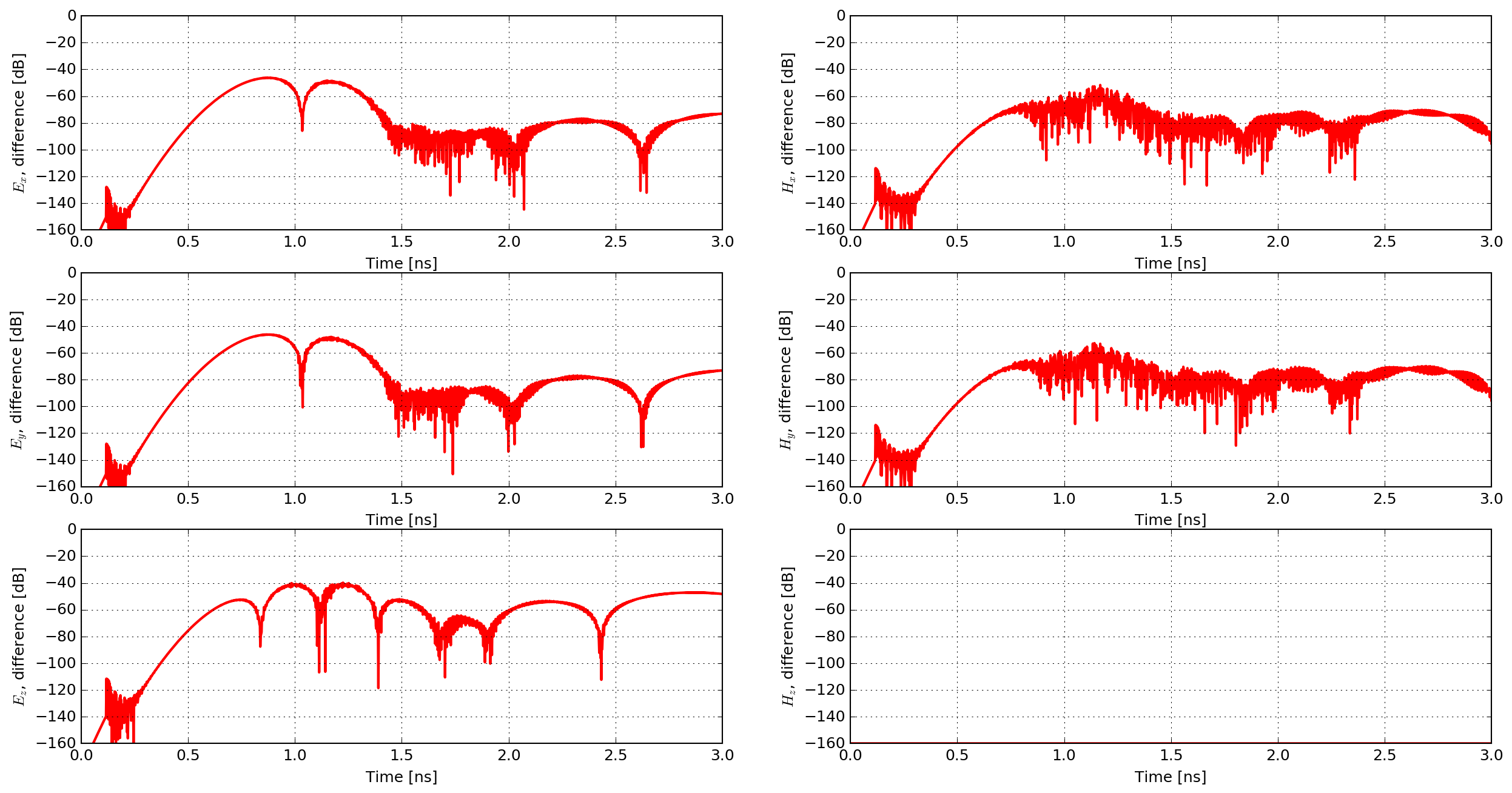
Fig. 47 Percentage differences between the modelled and analytical solutions.
The match between the analytical and numerically modelled solutions is excellent. The maximum difference is approximately 1%, which is observed in the Ez field component (the same direction as the Hertzian dipole source). The other electric field components exhibit maximum differences of approximately 0.5%, and the magnetic field components 0.25%.
Half-wave dipole in free space
See the section on antenna example models for the simulated s11 parameter and input impedance of a half-wave dipole antenna in free space. The resonant frequency and input impedance from the model agree very well with the theoretical predictions for a half-wave dipole antenna.